Out of proportion
The math of opinions
This post approaches the math of opinions by discussing its simplest example: how to understand whether something is fine or not. 5 developers is not a survey. 400 people of the specific universe might be. We all know this. We all forget this. That fuels endless discussions.
It's fine
Some years ago, I was managing a project where a CEO decided to short-circuit the usual development process and ask a developer directly to implement an absolutely terrible UI behavior. When I asked the developer about the eye-offending monstrosity he committed, he quickly blamed the CEO. When I asked the CEO about the animated horror he requested he said it was fine, claiming to have checked with five members of the team. Five of his employees and no written evidence. And no ticket. Obviously.
Not every CEO knows statistics. Turns out that there is a statistical method to determine whether something is fine or not. It's called a survey. We might be interested in determining the proportion of the relevant population that considers that something is fine. Because studying a population is rarely possible, we must accept studying only a sample, and infer the real proportion from the proportion found in the survey, hopefully with reasonable accuracy.
That's it.
A statistic is a mathematical function that maps a certain quantity X from n surveyed items of an N-sized population to a number: the Mean, the Median, the Standard Deviation, etc. Statistical inference is the process of estimating the statistics of X for the case n=N when in fact n << N. If we consider X=1 when "it's fine", and X=0 otherwise, the proportion we are looking for is the sample mean of X, where n is the number of customers surveyed and N is the universe of potential customers.
Developers on the payroll are not to be surveyed by the CEO when it comes to evaluating the software they are developing!
The rest is details.
The rest
In order to find the sample mean of X, we need to find the possible values k for the number of "it's fine" answers and assign a probability to each case. The variable representing these possible values will be called Y. Let's consider the number of people that say "it's fine" in the population is an unknown value K. As the survey goes on, the probability of finding "it's fine" answers decays slowly every time a fine answer is found and increases slightly every time a less-than-fine answer is found. This survey process is also known as sampling without replacement.
The probability that the j-th extraction results in "it's fine" (a success) is:
\(\displaystyle \frac{K - \text{successes so far}}{N - j} \)
whereas the probability of failure is:
\(\displaystyle \frac{N - j - (K - \text{successes so far})}{N - j} \)
For a sequence of k successes we will have the following terms in the numerator:
\(\displaystyle K(K-1)\dots(K-k+1) \cdot (N - K)(N-K-1)\dots(N-K-(n-k)+1) \)
and the following terms in the denominator:
\(\displaystyle N(N-1)\dots(N-n+1) \)
The probability for a generic sequence of survey results can be expressed as:
\(\displaystyle \frac{K(K-1)\dots(K-k+1) \cdot (N - K)(N-K-1)\dots(N-K-(n-k)+1)}{N(N-1)\dots(N-n+1)} \)
The numerators and denominators can be rewritten as combinations, at the cost of a left over term 1/C(n,k):
\(\displaystyle \frac{1}{\binom{n}{k}} \cdot \frac{\binom{K}{k}\binom{N-K}{n-k}}{\binom{N}{n}} \)
But because the sequence is generic for k successes and there are many possible sequences with the same number of successes, we need to multiply it precisely by coefficient C(n,k), which cancels the left over term. We arrived at the 300 year old Hypergeometric distribution:
\(\displaystyle P(Y=k) = \frac{\binom{K}{k}\binom{N-K}{n-k}}{\binom{N}{n}} \)
which in this case measures the probability of finding k "it's fine" answers in a population where K people think "it's fine". The estimated proportion is k/n.
Problem solved, right?
A much wanted simplification
The problem is still not solved because we don't know how good the estimation k/n is in relation to the real proportion p=K/N. And ideally, we would like a not too complicated solution.
Whenever the population is very large (e.g. in the magnitude of millions) compared to the sample we are able to collect (e.g., in the magnitude of hundreds) the expression for a generic sequence of survey results can be greatly simplified as:
\( \displaystyle \frac{K(K-1)\dots(K-k+1) \cdot (N - K)(N-K-1)\dots(N-K-(n-k)+1)}{N(N-1)\dots(N-n+1)} \simeq \left(\frac{K}{N}\right)^k \left(1 - \frac{K}{N}\right)^{n-k} \)
or, equivalently:
\( \displaystyle \frac{K(K-1)\dots(K-k+1) \cdot (N - K)(N-K-1)\dots(N-K-(n-k)+1)}{N(N-1)\dots(N-n+1)} \simeq p^k (1-p)^{n-k} \)
where p=K/N.
The fact that removing a small fraction of the population, little by little, as the survey advances, hardly influences the associated probabilities is something that connects with intuition, but can also be proven mathematically. We work under the assumption that even in the order of magnitude of respectable samples (hundreds of units) the approximation described above is valid.
As before, the sequence is generic for k successes and there are many possible sequences with the same number of successes. Once we multiply by the combinations coefficient C(n,k) we obtain the much simpler Binomial Distribution:
\( \displaystyle P(Y=k) = {\binom{n}{k}} p^k (1-p)^{n-k} \)
It is simple to verify that the expected value is given by:
\( \displaystyle E(Y) = np \)
and the Variance is given by
\( \displaystyle Var(Y) = np(1-p) \)
Samples aren't simple
We derived above a variable called Y, that counts the number of successes for a sequence of observations of the "It's fine" variable, called X. Y follows approximately the Binomial Distribution. Because we want to count the proportion of people that say "It's fine" rather than the number successes, we define a new variable W = Y/n. This variable follows what is usually called the Sampling Distribution. We can now use a property of the Variance to note that:
\( \displaystyle Var(W) = \frac{1}{n^2} Var(Y) = \frac{1}{n} p(1-p) \)
The corresponding Standard Deviation is then:
\( \displaystyle S(W) = \sqrt{\frac{p(1-p)}{n}} \)
This means the determination of the population proportion from the sample proportion shows dispersion, which we measure via the usual metric: the Standard Deviation. We expect dispersion to go away as we add more and more observations, the sample proportion slowly converging to the population proportion.
It is an interesting exercise to write the expression for W explicitly. It can be easily obtained by substituting w=k/n in the definition of Y, from which we find:
\( \displaystyle P(W = w) = \binom{n}{n w} p^{n w} (1-p)^{n(1-w)} \)
defined for
\( \displaystyle w = \left\{ 0, \, \frac{1}{n}, \, \frac{2}{n}, \, \dots, \, \frac{n-1}{n}, \, 1 \right\} \)
In formal terms, this expression does not introduce any new information - it expresses the same information as the Binomial Distribution followed by Y. But seeing its form and its domain explicitly written highlights one obvious fact that might not be obvious: the amount of possible different values for the estimated proportion is exactly n+1. That is, the proportion space is split into intervals of width 1/n which are very coarse grained for low n. For the n=5 anecdote, the possible values for the estimated proportion could be no others than {0, 0.2, 0.4, 0.6, 0.8, 1 }. If the real proportion is, say 0.3, the nearest observable sample values (0.2 and 0.4) are 0.1 units off.
That is, on top of the natural dispersion that causes small samples to not represent the population well, there is also a problem of granularity of representation. This problem too, fades away with larger samples, because as n increases the domain of W becomes denser. With n=5 possible values are separated by spaces of 0.2 (or 20%, in percentage) whereas for n=20 possible values are separated by 0.05 (or 5% in percentage) and for n=100, possible values are separated by 0.01 (or 1%, in percentage). The maximum error introduced due to lack of representation granularity would be 0.1, 0.025 and 0.005 or, in percentages, 10%, 2.5%, and 0.5%, respectively.
In general, the granularity error is given by:
\( \displaystyle E_g = \frac{1}{2n} \)
so no sample of size n can guarantee an error smaller than the above, regardless of dispersion. In other words:
\( \displaystyle E \ge \frac{1}{2n} \)
This idea alone already sets a basic minimum requirement for the sample size:
\( \displaystyle n_g \ge \frac{1}{2E} \)
where E is the tolerable error.
We will see later that this condition is necessary but not sufficient. The reason is that the granularity problem decreases with the inverse of n, faster than the dispersion caused by sampling randomness, which fades out with the inverse of the square root of n. Still, this simple criterion is enough for ruling out small samples (e.g. n<10) where the granularity error is significant.
Error and Confidence
We have seen from the expression for S(W), that the dispersion on the determination of the proportion depends on the population proportion itself. If the population proportion is 0 or 1, dispersion will be 0, because all population items are equal. On the other hand, it is easy to see that dispersion is maximized when p=1/2.
Let that sink in for a moment: the determination is not straightforward, because dispersion decays slowly, with the inverse of the square root of n, and we expect it to be harder when the population's opinions are split 50/50. In order to prepare a survey we must be ready for the worst case: p=1/2.
But how? Ideally, we would find a way to locate the population proportion within an acceptable bound around the estimated proportion.
Let's use variable W to formalize the desired result:
\( \displaystyle P\left(\frac{k}{n} - E \le p \le \frac{k}{n} + E\right) \ge 1 - \alpha \)
This condition says that with probability 1-alpha the population proportion is inside the estimated proportion +-E , where E is the error we decided to tolerate. This probability is usually called the Confidence Level.
We can break it down in two separate conditions:
\( \displaystyle P\left(\frac{k}{n} \le p + E\right) \ge 1 - \frac{\alpha}{2} \)
\( \displaystyle P\left(\frac{k}{n} \ge p - E\right) \ge 1 - \frac{\alpha}{2} \)
In order to consider the worst case dispersion we set p=1/2. Because the Binomial Distribution becomes symmetric in that case, the two expressions above contain the same information:
\( \displaystyle P\left(\frac{k}{n} \le \frac{1}{2} + E\right) \ge 1 - \frac{\alpha}{2} \)
This is the generic expression that we need. Once we decide on the tolerated error and the probability we can theoretically determine the minimum necessary sample size. The required sample size will be larger for larger values of the required probability and for smaller values of the tolerated error. For E = 0.05 and alpha = 0.05 we would find:
\( \displaystyle P\left(k \le 0.55n \right) \ge 0.975 \)
This is a simple probability condition, with an open parameter - n - to be determined. Here is, however, a minor practical problem: the equation above can not be solved for n in a closed form.
Luckily, looking for the right value of n takes less than half a second on a computer. Here is an example program that calculates the minimum sample size:
#!/usr/bin/python3

from scipy.stats import binom

MAX_SAMPLE=100000

def verify_sample_size(n, E, alpha):

    # we calculate for the proportion that maximizes dispersion, i.e., the worst case
    p = 0.5

    # k_upper is the largest integer outcome within the allowable margin E
    k_upper = int(n * (p + E))

    # Evaluate the cumulative probability between 0 and k_upper for p=0.5 and generic E
    coverage_prob = binom.cdf(k_upper, n, p)

    # Must satisfy two-sided coverage (1 - alpha/2); returns True/False
    return coverage_prob >= (1 - alpha / 2)


for n in range(1, MAX_SAMPLE):
    result = verify_sample_size(n, 0.05, 0.05)

    if result:
        print("the minimum necessary sample size is", n)
        exit()check

print("no value found for sample below", MAX_SAMPLE)
In 2026, running this kind of program is as natural as pressing the square root button in a Casio calculator from the 90's.
A slightly improved version of this code can be found here. This improved version compensates for the optimistic nature of the example code above - the binomial coverage isn’t monotone, which needs to be compensated by testing larger values of n until we are sure the coverage stabilizes (still an effect of granularity!). It also allows us to explore the relationship between tolerated error, confidence level and sample size:
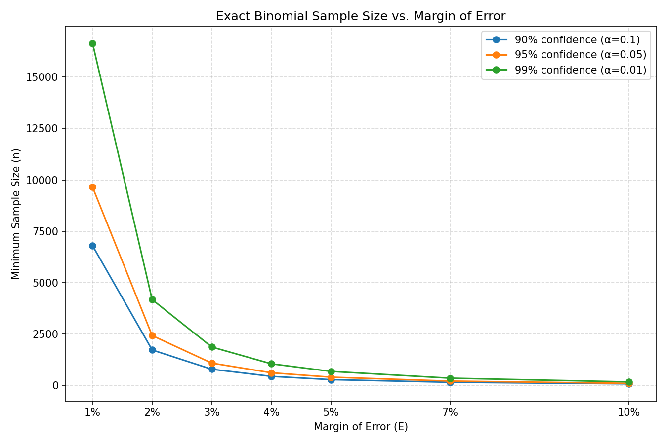
From here, because we have seen the expression for the Standard Deviation of the sample mean, we can take an educated guess at a candidate function for numerical fitting:
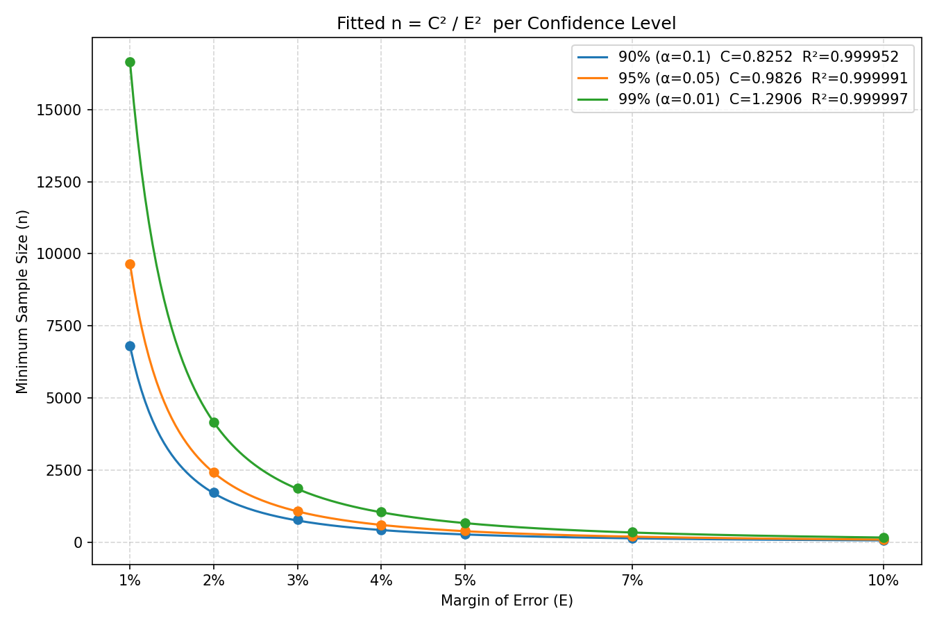
It becomes clear that the dispersion error is given by:
\( \displaystyle E_d \simeq \frac{C}{ \sqrt{n} } \)
where C is a constant determined by the confidence level. From here, noticing that the dispersion error fades slower than the granularity error, as n grows, we deduce a stricter condition for the sample size:
\( \displaystyle n \ge \frac{C^2}{E^2} \)
For the industry standard confidence level 95% - that is (1 - alpha = 0.95) - an approximate formula becomes possible:
\( \displaystyle n \ge \frac{0.97}{E^2} \)
This formula returns n=388 for an error of 5% (E=0.05). Running the provided python snippet directly would yield n=371 whereas running the improved version would result in n=399.
As far as I can see, none of them returns 5 developers on your payroll!
The underlying math
ONGOING
Conclusion
If you want to know if something is fine or not, it is a good idea to ask approximately 400 people from the right population. The explanation, though, may have blown out of proportion.