Published on 2026-01-30 by GCH

The Linux load average

What is the Linux load average?

This is not exactly an orphan question but, as happens with other questions I try to address in this blog, it is surrounded by confusion. Whenever one begins discussing load averages, confusion steps in and refuses to leave. I will try to provide an explanation that is "as simple as possible, but not simpler" and also short enough to be worth reading.

Context

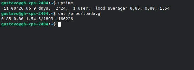
We sometimes see the load average values of a system in the output of the uptime command or by inspecting /proc/loadavg:

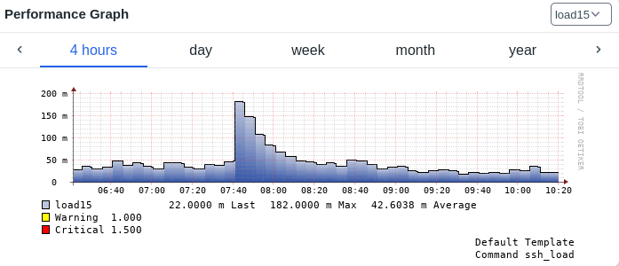
We often see plots of load average values inside monitoring systems:

This post will bring meaning to these images.

Definition 1

We will call the instantaneous load of a system the number of tasks - processes and threads - that are willing to run at a given time t.

Tasks willing to run are tasks in state R or D. That is, they are either actually running or blocked on some resource (CPU, I/O, ...) waiting for an opportunity to run. The instantaneous number of such tasks can be determined using the ps command:

ps -eL h -o state | egrep "R|D" | wc -l

To be clear: tasks that want to run but are waiting for a CPU core to be available or that are waiting for data from the disks / network also count as instantaneous load.

(see footnote [1] for more info on this)

Definition 2

We will define the load average of a system as a specific averaging function of the instantaneous load value and the history of previous values. In particular, for Linux systems, the recursive weighted average:

\( a_t= Ca_{t-1} + (1- C)l_t \)

where

\( C = e^{-5/60A} \)

has been adopted.

In the previous expressions l_t is the instantaneous load, from definition 1, and parameter A takes the values of 1, 5 and 15. The three sequences, corresponding to the three possible values of A, are called the 1m, 5m and 15m load average, respectively.

For A=0 we would find:

\( a_t = l_t \)

therefore, recovering definition 1 - the instantaneous load is simply the 0m load average.

Historically, the load average values were calculated by the kernel every 5 seconds. In the current kernels there are some nuances related to the sampling but nothing has changed conceptually.

Discussion

First of all, we should stress that the load average from definition 2 is just a generalization of definition 1.

While their values are similar in nature, the larger the value of A, the lower the contribution of the instantaneous load compared to the contribution of the historic load average value. The main purpose of using an "averaging" function is the smoothening of fast oscillations that could render human inspection of load values nearly impossible. The timespan of that smoothening effect is influenced by parameter A. In mathematical terms a_t applies Exponential smoothing to l_t.

The recursive sequence for a_t is simple but its ultimate meaning might not be evident at a first glance. With a bit of work we can transform it into an explicit sequence:

\( a_t= C^t a_{0} + (1-C)\sum\limits_{j = 0}^{t-1} C^j l_{t-j} \)

Since, by definition, a₀=l₀ we get:

\( a_t= C^t l_{0} + (1-C)\sum\limits_{j = 0}^{t-1} C^j l_{t-j} \)

which can also be expressed as:

\( a_t= C^t l_{0} + (1-C)\sum\limits_{j = 1}^{t-1} C^j l_{t-j} + (1-C)l_t \)

That is, the sequence is composed by three terms:

the initial instantaneous load value multiplied by a coefficient that decays to exponentially to zero; this term disappears quickly as time passes
all other past instantaneous load values multiplied by coefficients that make them loose importance exponentially, as their index t-j goes from the present to the past
the current load value multiplied by (1-C)

Since the first term decays quickly, in order to study the importance of the past instantaneous load values we must focus on the second term.

First we note that the sequence of coefficients:

\( C^1, C^2, ... C^{t-1} \)

is a geometric progression and thus decays by a fixed fraction with each iteration.

Now let's suppose we want to check how many iterations it takes for this sequence of coefficients to decay from C to C divided by a constant k. If we write:

\( C^j = C/k \)

we will find:

\( j-1 = - {{ln(k)} \over {ln(C)}} \)

where j-1 is the number of iterations connecting j sampling moments. Given that there are 5 seconds between samples, this is equivalent to saying:

\( t_{1/k} = - 5 {{ln(k)} \over {ln(C)}} \)

If we now insert the definition of C, we get:

\( t_{1/k} = ln(k) 60A \)

Finally, by setting k=e we obtain:

\( t_{1/e} = 60A \)

From here we see that the Xm load average is the instantaneous load exponentially smoothed in such a way that the importance of the coefficients applied to the historical load values reduces to 1/e in X minutes. The mysterious coefficients at the definition of a_t are now explained!

Because e =~ 2.7, a reduction to 1/e of the initial value is aproximately a reduction of 63%. It is also easy to verify that a reduction of 95% happens in 3, 15 and 45 minutes for the 1m, 5m and 15m load averages, respectively.

The Linux kernel provides these three distinct load averages so that users can analyze how the system responds at different timescales to sudden changes in instantaneous load. All of them converge the to instantaneous load value - at different rates - if it stabilizes. Which of these sequences is most useful depends on the practical situation.

Let's go for a hands-on exercise.

The load average can be calculated with a simple bash script, using definitions 1 and 2, just as the Linux kernel does (see kernel source). Here is the example output of one such calculation that estimates the 1m load average and compares it to the calculation performed by the Linux kernel:

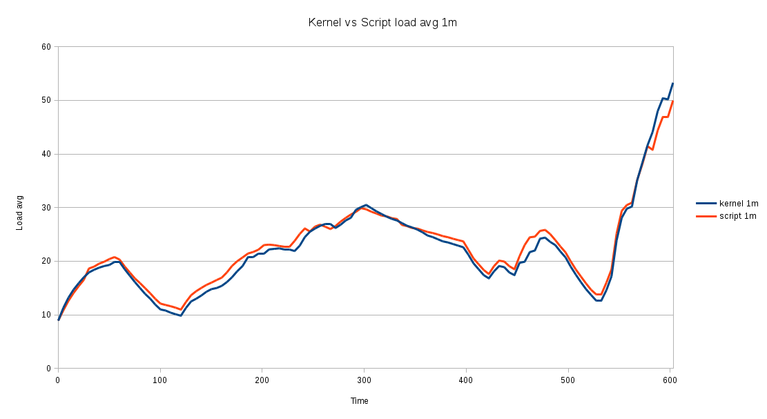
This result confirms that definitions 1 and 2 are correct, as the difference between the script-based calculation and the kernel calculation is negligible.

The same script also allows us to evalute the different load metrics on a real system that is initially running on a "baseline load with fluctuations" regime and is then put to stress during 5.5 minutes, after which it returns to its initial state:

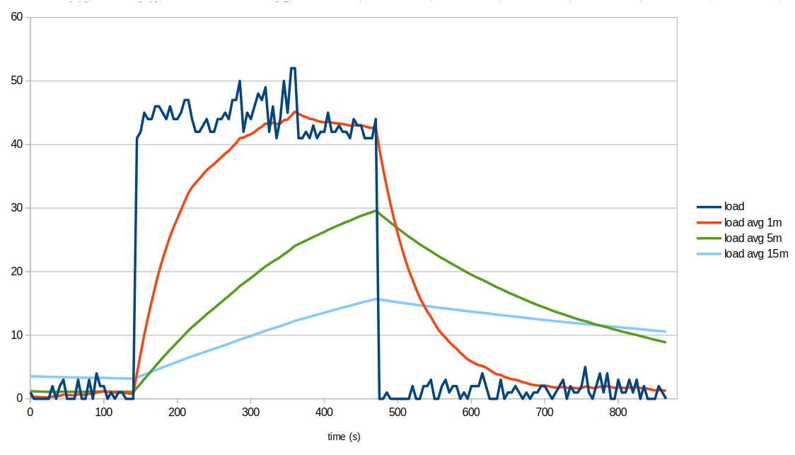
We can clearly see that the load average metrics smooth short-lived fluctuations (multiple cycles per minute). They also respond slowly to transitions between sustained load regimes. In this example, the baseline load stayed elevated for about 5.5 minutes, and only the 1m load average had enough time to converge to the higher instantaneous load and then return toward the baseline. It took roughly three minutes to approach the new level in each direction, while the 5m and 15m load averages mostly produced intermediate values because the pulse was short relative to their smoothing windows.

If the higher-load pulse had been shorter, none of the load averages might have moved much. In practice, load averages are useful for showing load patterns on timescales of minutes - faster variations are strongly attenuated and very short pulses are mostly smoothed out.

Now that frequencies have been dealt with, let's come back to the load values. We now need to argue that there is no such thing as a too high load average, in absolute terms. In fact, the number of tasks that are willing to run on a given system depends on:

the architecture of the software that is running (is it mostly monolithic? or prone to spawn many processes? how dependent are such processes between each other?)
the CPU throughput requested by the software that is running
the I/O throughput requested by the software that is running
the CPU performance of that system
the I/O performance of that system
the number of available cores

Therefore, we can only say "the load average is too high on that system" if we know the "normal value for that system". The "normal value" is an empirically discovered value under which that system usually runs and is known to perform acceptably. The normal value could well be 2 for a server with a low number of cores that runs an interactive web application, or could be 50 for a server that runs (non-interactive) numeric simulations jobs during the night.

Furthermore...

for the same requested I/O effort and the same hardware, a software implementation that spreads the computation across many processes or threads will generate a higher load average; even though the actual throughput is the same, 10 processes trying to write 10MB each, on an I/O starved system, generate a higher load average than one process trying to write 100MB on the same system.
given a certain software program that sets all the existing CPU cores to 100% while running on a specific machine, its execution on a system with smaller a number of cores, or slower cores, will generate a higher load average; whether that higher load is a problem or not depends on the use case (if it means your numeric simulation or your file server backup takes 10 more minutes during the night but will still be ready in the morning then no harm is done).

Load average vs CPU usage

As we have seen, load average values don't have an absolute numerical meaning unlike CPU usage values, which are expressed in % of CPU time:

%usr - time spent running non-kernel code. (user time, including nice time)
%sys - time spent running kernel code. (system time)
%wait - time spent waiting for I/O.
%idle - time spent idle.

Note: %wait is not an indication of the amount of I/O going on - it is an indication of the extra %usr time that the system would show if I/O transfers weren't delaying code execution.

For systems running below their limits, CPU usage values are much more useful than load average values, since their numeric interpretation is universal. But once limits are hit, i.e., CPU %idle time becomes nearly zero, load average values allow us to see how much off the limits the system is running... once we establish a baseline, which is the normal load average for that system (software+hardware combination).

Summary of true statements

If all system cores are running at %sys+%usr=100 the instantaneous load is equal to or higher than the number of cores.
The instantaneous load being higher than the number of cores doesn't mean all cores are running at %sys+%usr=100, since many processes may be I/O waiting (state D).
The instantaneous load being higher than the number of cores implies that the system can't be mostly idle; at least some of the cores will be seen for a relevant amount of the time in sys, usr or wait states.
A system can be slow/unresponsive even with an instantaneous load below the number of cores because a small number of I/O intensive processes may become a bottleneck.
In a pure CPU intensive scenario (negligible I/O, no processes in state D) where %idle > 0, the instantaneous load is equal to ((100 - %idle)/100) * NCORES; for instance, on a 4 core system at steady %sys+%usr=90 we would have an instant load of ((100-10)/100)*4 = 3.6.

Statement 5 can be easily tested by running:

stress -c X

while looking at the output of top on a different terminal, waiting for the 1m load average to stabilize. It is trivial to see that the above formula holds up to X=NCORES, which will cause %idle=0.

Note on Hyperthreading: We haven't discussed Hyperthreading, or the equivalent AMD feature, to avoid complicating the discussion but where above we say NCORES, it could be the number of virtual CPUs, including CPU threads. Of course, each additional % usage on the second thread of an already busy core doesn't yield a proportional throughput.

Footnotes

[1] - The same result should be obtainable by parsing /proc/loadavg (4th field) or /proc/stat (procs_running, procs_blocked) but I have seen from experience that multiple processes in state D are shown by ps but not counted on /proc/loadavg and that neither /proc/loadavg (4th field) nor /proc/stat include threads in the task counters, even though they are taken into account in the load average numbers exposed by the kernel.

References

The load average bible in three volumes: